The base classes of paintbox

The spectral energy distribution (SED) of galaxies can be decomposite into different parts, such as the light from the stars, the emission lines from the gas, and the attenuation of the light as a whole owing to dust absorption. Similarly, paintbox uses different ingredients to build a model for the SED that com be combined to produce a SED model. We start with two base classes used to handle models in the form of templates, NonParametricModel and ParametricModel, and then we show the auxiliary classes used to modify the SED in general.

import os
import numpy as np
import astropy.units as u
from astropy.modeling import models
from astropy.io import fits
from astropy.table import Table, vstack
import matplotlib.pyplot as plt
import paintbox as pb
from paintbox import utils
from ppxf import ppxf_util, miles_util

Non-parametric models

The SED of galaxies can be modeled as a superposition of templates, i.e., given a set of SED models A, an observed spectrum (or some parts of it) can described as an weighted sum of models in A. In this case, the problem of modeling the SED becomes to find an optimal set of weights. This method have been extensively explored by some tools such as ppxf and Starlight. For instance, in the modeling of emission lines, ppxf provides a simple tool to produce templates of the most important optical lines, as shown below.

# Generating an wavelength array spaced logarithmically with
# fixed velocity scale
wrange = [4000, 7000]
velscale = 30 # Velocity shift between pixels
FWHM = 2.8 # Resolution of the observation

# Simple tool to get velocity dispersion with fixed velscale within a given range
wave = utils.disp2vel(wrange, velscale)
logwave = np.log(wave)

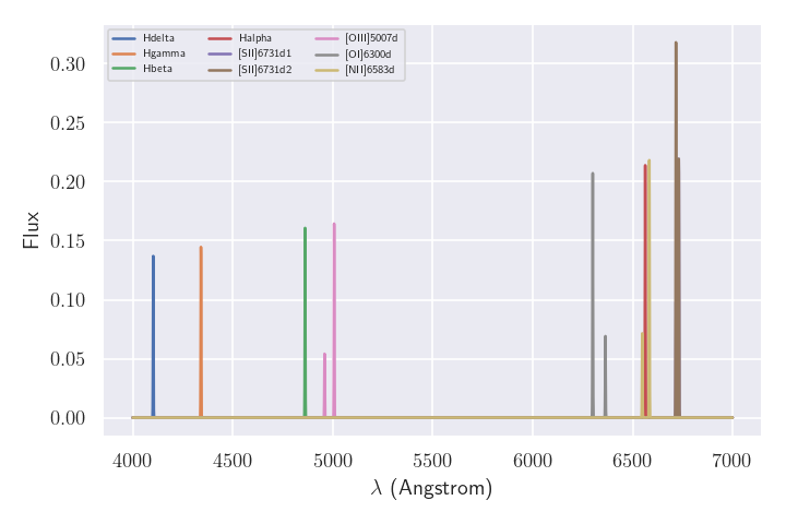
gas_templates, gas_names, line_wave = ppxf_util.emission_lines(
        logwave, [wave[0], wave[-1]], FWHM,
        tie_balmer=False, limit_doublets=True)
gas_names = [_.replace("_", "") for _ in gas_names] # Removing underlines from names
fig = plt.figure(figsize=(8, 6))
for i in range(len(gas_names)):
    plt.plot(wave, gas_templates[:,i], label=gas_names[i])
plt.legend(ncol=5, prop={"size": 8})
plt.xlabel("$\lambda$ (Angstrom)")
plt.ylabel("Flux")
plt.show()

Emission lines included in gas templates:
['Hdelta' 'Hgamma' 'Hbeta' 'Halpha' '[SII]6731_d1' '[SII]6731_d2'
 '[OIII]5007_d' '[OI]6300_d' '[NII]6583_d']

In paintbox, we can also use templates as those shown above using the NonParametricModel class. For instance, to use the emission line templates shown above, we just need to do the following:

# Creating paintbox component
emission = pb.NonParametricModel(wave, gas_templates.T, gas_names)
print("Name of the parameters", emission.parnames)
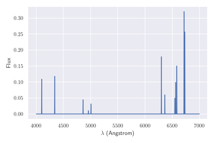
# Generating some random flux for each emission line
theta = np.random.random(len(gas_names))
print("Random fluxes of emission lines: ")
print(*zip(emission.parnames, theta))
fig = plt.figure(figsize=(8, 6))
plt.plot(wave, emission(theta))
plt.xlabel("$\lambda$ (Angstrom)")
plt.ylabel("Flux")
plt.show()

Name of the templates:  Hdelta, Hgamma, Hbeta, Halpha, [SII]6731d1, [SII]6731d2, [OIII]5007d, [OI]6300d, [NII]6583d

Now, the emission object above can be called to produce a linear combination of all templates by providing a set of weights, given in the order indicated by the parnames parameter, as indicated in the example below.

# Generating some random flux for each emission line
theta = np.random.random(len(gas_names))
print("Random fluxes of emission lines: ")
print(*zip(emission.parnames, theta))
fig = plt.figure(figsize=(8, 6))
plt.plot(wave, emission(theta))
plt.xlabel("$\lambda$ (Angstrom)")
plt.ylabel("Flux")
plt.show()

In practice, this class can be used in different ways, including emission line modeling, sky and telluric removal / correction, and also with stellar population models. Moreover, NonParametricModel compononents can be combined with any SED components in paintbox, and they can be modified later to include, e.g., kinematics and dust attenuation.

Parametric models

In several applications, we are interested in the determination of the parameters involved in the modeling of the SED, for instance, the age or the metallicity of a stellar population model that better describes some observations. The NonParametricModel class above can be used for that purpose, of course, but the problem of determining the correct weights becomes more difficult as we include more templates. One alternative is to restrict the model to a given (small) number of spectra, e.g., assuming a single stellar population approximation, and then search for a single spectrum that describe the observations. This can be performed by interpolating the models according to their parameters, and it is the main usage of the ParametricModel class. In the example below, we use a set of theoretical stellar models from Coelho (2014), (which you can download here) to demonstrate how to use this class to interpolate spectra in a stellar library.

import os

from astropy.io import fits
from astropy.table import Table, vstack

models_dir = "s_coelho14_sed"
# Getting parameters from file names
model_names = os.listdir(models_dir)
# Get dispersion from the header of a file
filename = os.path.join(models_dir, model_names[0])
crval1 = fits.getval(filename, "CRVAL1")
cdelt1 = fits.getval(filename, "CDELT1")
n = fits.getval(filename, "NAXIS1")
pix = np.arange(n) + 1
wave = np.power(10, crval1 + cdelt1 * pix) * u.micrometer
table = []
templates = np.zeros((len(model_names), n))
for i, filename in enumerate(model_names):
    T = float(filename.split("_")[0][1:])
    g = float(filename.split("_")[1][1:])
    Z = 0.1 * float(filename.split("_")[2][:3].replace(
        "m", "-").replace("p", "+"))
    alpha = 0.1 * float(filename.split("_")[2][3:].replace(
        "m", "-").replace("p", "+"))
    a = np.array([T, g, Z, alpha])
    t = Table(a, names=["T", "g", "Z", "alpha"])
    table.append(t)
    templates[i] = fits.getdata(os.path.join(models_dir, filename))
table = vstack(table) # Join all tables in one
# Use paintbox to interpolate models.
star = pb.ParametricModel(wave, table, templates)
print("Parameters: ", star.parnames)
print("Limits for the parameter: ", star.limits)
theta = np.array([6500, 3., -0.1, 0.1])
fig = plt.figure(figsize=(8, 6))
plt.semilogx(wave, star(theta))
plt.xlabel("$\lambda$ ($\mu$m)")
plt.ylabel("Flux")
plt.show()

Parameters:  ['T', 'g', 'Z', 'alpha']
Limits for the parameter:  {'T': (3000.0, 26000.0), 'g': (-0.5, 5.5), 'Z': (-1.3, 0.2), 'alpha': (0.0, 0.4)}

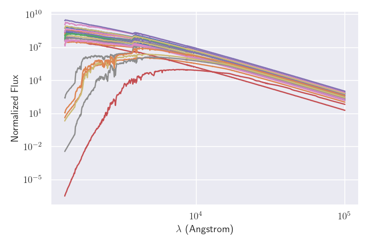
The above code illustrates how to prepare the data for paintboxingestion for a particular case, but we notice that the ParametricModel class require only three arguments, the wavelength array (one for each spectral element), an astropy.table.Table object that contains the parameters of the model, and a 2D numpy.ndarray with the correspondent models for each table row. There is no single standard of distribution for model files, and such preliminary preprocessing requires some tweaking accordingly. For some stellar population models, including Miles and CvD models, paintbox provides additional utility classes that simplify this process further. Please check the building_models tutorial and documentation for more details.

Polynomials

Polynomials are often used to offset the models in match the observations. Thepaintbox uses Legendre polynomials, which can be used as indicated below.

import numpy as np
import paintbox as pb
import matplotlib.pyplot as plt

wave = np.linspace(5000, 7000, 2000)
degree = 10
poly = pb.Polynomial(wave, degree)
print(f"Parameter names: {poly.parnames}")
theta = np.random.random(degree + 1)
fig = plt.figure(figsize=(8, 6))
plt.plot(wave,poly(theta))
plt.xlabel("$\lambda$ (Angstrom)")
plt.ylabel("Flux")
plt.savefig("polymial_example.png")
plt.show()

Parameter names: ['p_0', 'p_1', 'p_2', 'p_3', 'p_4', 'p_5', 'p_6', 'p_7', 'p_8', 'p_9', 'p_10']

Notice that the default behaviour of the Polynomial class includes the zero-order term, such that a polynomial of order n requires n+1 parameters. The zero order polynomial can be suppressed using the option zeroth=False.

Extinction laws

Currently, paintboxsupports two extinction laws, CCM89 for the relation used by Cardelli, Clayton and Mathis (1989) for the Milky Way, and C2000 proposed by Calzetti et al. (2000). In both cases, paintboxreturns the attenuated flux according to a dust screen model,

\(\frac{f_\lambda}{f_\lambda^0}= 10^{-0.4 A_V \left (1 + \kappa_\lambda / R_V\right )}\),

where the free parameters are the total extinction \(A_V\) and the total-to-selective extinction \(R_V\). These models can be used as follow:

import numpy as np
import paintbox as pb
import matplotlib.pyplot as plt

wave = np.linspace(3000, 10000)
ccm89 = pb.CCM89(wave)
c2000 = pb.C2000(wave)
theta = np.array([0.1, 3.8])
fig = plt.figure(figsize=(8, 6))
plt.semilogx(wave, ccm89(theta), label="CCM89")
plt.semilogx(wave, c2000(theta), label="C2000")
plt.xlabel("$\lambda$ (Angstrom)")
plt.ylabel("$f_\lambda / f_\lambda^0$")
plt.legend()