Stellar population models

Paintbox is particularly designed to model the observed spectrum, i.e., the flux from stars as a function of the wavelength, of galaxies where stars are not individually resolved. In these cases, the most important ingredient to describe the stellar features in observations are stellar population models, which describe the properties of an emsemble of stars with different properties, e.g., ages, metallicities, etc. Several groups of astronomers distribute their models for free for users, either publicily or under request. However, there is no single standard way of distributing stellar population models, so we have to prepare the data from the models before using paintbox. Moreover, in practical applications, we also require the models to be tunned according to the scientific requirements of the modeling as a way to minimize the (often expensive) number of computations depending on the resolution of the data.

EMILES

Stellar populations models from the MILES library can be obtained in a variety of ways in their website. For this example, we will use the packages astropy to handle FITS fiels and tables, and the [pPXF](ppxf for rebinning the data to a logarithmic scale.

import os

import numpy as np
from astropy.io import fits
from astropy.table import Table
from ppxf import ppxf_util

For this example, we will use a set of single stellar population (SSP) templates of the E-MILES models (version 11) produced with BASTI isochrones and assuming a Chabrier initial mass function, which can be downloaded in a tarball from their public ftp link available in their website (EMILES_BASTI_BASE_CH_FITS.tar.gz, 95 Mb). After downloading the data, it is necessary to unpack the tarfile (preferentially into a subdirectory, which we name emiles_v11), containing the 636 SSP spectra in this case.

emiles_dir = "/home/kadu/Dropbox/SSPs/emiles_v11"
w1 = 2600 # Minimum wavelength
w2 = 10000 # Maximum wavelength

We can use the MILES name convention to read the files with the models.

def miles_filename(specrange, imf, imfslope, metal, age):
    """ Returns the name of a fits file in the MILES library according
    to the name convention. """
    msign = "p" if metal >= 0. else "m"
    azero = "0" if age < 10. else ""
    return "{0}{1}{2:.2f}Z{3}{4:.2f}T{5}{6:02.4f}" \
            "_iTp0.00_baseFe.fits".format(specrange, imf, \
            imfslope, msign, abs(metal), azero, age)

Below we produce a list containing all the spectra that we are going to use in our analysis (filenames), and we also produce an astropy Table object storing the parameters of the files.

specrange = "E" # options: "E", "M", "B", "R", "C"
imf = "ch" # options: "un", "bi", "ku", "kb", "ch"
imfslope = 1.3
# Values of metallicities and ages available for BASTI isochrones
Zs = np.array([-0.96, -0.66, -0.35, -0.25, 0.06, 0.15,  0.26,  0.4])
Ts = np.linspace(1., 14., 27) # Using only ages > 1 Gyr
ssps_grid = np.array(np.meshgrid(Ts, Zs)).T.reshape(-1, 2)
nssps = len(ssps_grid)
filenames = []
for t, z in ssps_grid:
    filenames.append(miles_filename(specrange, imf, imfslope, z, t))
params = Table(ssps_grid, names=["T", "Z"])

We use the information in the header of one spectrum to determine the wavelength range (which is always the same for a given set of models). Notice that the wavelength range covered by the EMILES models is large (from the near-UV to the IR).

h = fits.getheader(os.path.join(emiles_dir, filenames[0]))
wave = (h['CRVAL1'] + h['CDELT1'] * (np.arange((h['NAXIS1'])) + 1 - h['CRPIX1']))

Finally, we need to trim and/or rebin the model spectra. We need to trim the data to cover only the spectral region of the observed data. Notice, however, that we should always have extra coverage in the models, preferentially on both edges of the spectra, if we are also modeling the kynematics of the galaxy, and also to avoid problems at the edges of the models owing to convolutions (below I use 500 Angstrom, but this can be optimized for a galaxy according to their redshift). We may also rebin the data, either to have the same wavelength dispersion of the observations, or to a logarithmic scale to model the kinematics. We use the pPXF for this purpose, assuming a velocity scale for the rebinning of 200 km/s.

velscale = 200
extra_wave = 500
idx = np.where((wave >= w1 - extra_wave) & (wave <= w2 + extra_wave))
wave = wave[idx] # Trimming wavelength array

# Using first spectrum to get array size after rebbining
flux = fits.getdata(os.path.join(emiles_dir, filenames[0]))[idx]
wrange = [wave[0], wave[-1]]
newflux, logLam, velscale = ppxf_util.log_rebin(wrange, flux,
                                                 velscale=velscale)
# Loop to trim and rebin spectra
ssps = np.zeros((nssps, len(newflux)))
for i, filename in enumerate(filenames):
    flambda = fits.getdata(os.path.join(emiles_dir, filename))[idx]
    flux_log = ppxf_util.log_rebin(wrange, flambda, velscale=velscale)[0]
    ssps[i] = flux_log

Now, we just need to store the processed data into a FITS file.

hdu1 = fits.PrimaryHDU(ssps)
hdu1.header["EXTNAME"] = "SSPS"
hdu2 = fits.BinTableHDU(params)
hdu2.header["EXTNAME"] = "PARAMS"
hdu3 = fits.BinTableHDU(Table([logLam], names=["loglam"]))
hdu3.header["EXTNAME"] = "WAVE"
hdulist = fits.HDUList([hdu1, hdu2, hdu3])
output = "emiles_chabrier_w{}_{}_vel{}.fits".format(w1, w2, velscale)
hdulist.writeto(output, overwrite=True)

In this particular example, we will obtain a multi-extension FITS file named “emiles_chabrier_w2600_10000_vel200.fits”, which contains the 2D array with the models, a parameter table, and an 1D array with the wavelength array. Notice that, in practice, if often necessary to degrade the model spectra to match the resolution of the observations, which can be performed with the task paintbox.utils.broad2res.

Using CvD stellar population models

Models from the Conroy and van Dokkum (2012) and Conroy et al. (2018), a.k.a. CvD models, can be obtained under request to the authors, and are not distributed together with paintbox. Similar to the MILES models, CvD are also distributed as SSP models with varying ages, metallicities, and IMFs, but also provide response functions that allow the variation of several individual elements, e.g., C, N, O, Mg, Si, Ca, Ti, and Fe. In this cases, To handle these models, we use the utility class CvD18, built from the basic paintbox classes, to handle the input files and produce spectra with any combination of parameters.

import os

import numpy as np
from paintbox.utils import CvD18, disp2vel
import matplotlib.pyplot as plt

# Defining an arbitrary wavelength region
w1, w2 = 5000, 9000 # Setting the wavelength window
sigma = 300 # Velocity dispersion of the output models
wave = disp2vel([w1, w2], sigma)
outdir = os.path.join(os.getcwd(), "CvD18_tutorials")
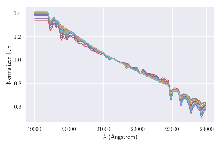
elements = ["Mg", "Na"] # Simple model with only two elements
ssp = CvD18(wave, sigma=sigma, store=outdir, elements=elements)
# Plotting n random models
fig = plt.figure(figsize=(8, 6))
n = 20
print("Model allowed ranges")
print(ssp.limits)
print("List of parameters of model")
print(ssp.parnames)
for i in range(n):
    theta = np.array([np.random.uniform(ssp.limits[p][0], ssp.limits[p][1])
                      for p in ssp.parnames])
    v = ssp(theta)
    plt.plot(wave, ssp(theta))
plt.xlabel("$\lambda$ (Angstrom)")
plt.ylabel("Normalized flux")

Processing SSP files: 100%|██████████| 35/35 [01:17<00:00,  2.21s/it]
Preparing response functions: 100%|██████████| 25/25 [00:14<00:00,  1.69it/s]

Model allowed ranges
{'Z': (-1.5, 0.2), 'Age': (1.0, 13.0), 'x1': (0.5, 3.5), 'x2': (0.5, 3.5), 'Mg': (-0.3, 0.3), 'Na': (-0.3, 0.9)}
List of parameters of model
['Z', 'Age', 'x1', 'x2', 'Mg', 'Na']

Please check out the documentation for the CvD18 class to set this class to work in your computer using the libpath keyword.

Visualizing response functions

To CvD18 class allows the access to all response functions used in an instance. Below we use the response function of iron, magnesium and titanium to reproduce figure 8 of Conroy et al. (2018).

import os

import numpy as np
import paintbox as pb
from paintbox.utils import disp2vel, CvD18
import matplotlib.pyplot as plt

wave = disp2vel([3800, 7000], 100)
sigma = 300 # Velocity dispersion of the output models
elements = ["Fe", "Mg", "Ti"]
outdir = os.path.join(os.getcwd(), "CvD18_tutorials")
ssp = CvD18(wave, sigma=sigma, outdir=outdir, elements=elements)
fig = plt.figure(figsize=(12, 8))
for i, element in enumerate(elements):
    rf = ssp.response_functions[element]
    # Upper panels with fixed metallicity
    Z = 0.2
    abund = rf.limits[element][1]
    ages = [1, 5, 13]
    ax = plt.subplot(2, len(elements), i+1)
    for age in ages:
        theta = np.array([Z, age, abund])
        ax.plot(wave, (rf(theta) - 1) * 100, label=f"{theta}")
        ax.legend(title=f"[Z, age, {element}]", prop={"size": 7})
    ax.set_xlabel("$\lambda$ (Angstrom)")
    ax.set_ylabel("ratio (\%)")
    ax.text(0.12, 0.12, element, fontsize=16, transform=ax.transAxes)
    # Lower panels with fixed age
    age = 5
    Zs = [-1.5, -1, -0.5, 0, 0.2]
    ax = plt.subplot(2, len(elements), i+4)
    for Z in Zs:
        theta = np.array([Z, age, abund])
        ax.plot(wave, (rf(theta) - 1) * 100, label=theta)
    ax.set_xlabel("$\lambda$ (Angstrom)")
    ax.set_ylabel("ratio (\%)")
    ax.legend(title=f"[Z, age, {element}]", prop={"size": 7}, ncol=2)
    ax.text(0.12, 0.12, element, fontsize=16, transform=ax.transAxes)
plt.tight_layout()